
\(\def\blambda{\boldsymbol \lambda}\) \(\def\bX{\boldsymbol X}\) \(\def\N{\mathbb N}\) \(\def\P{\mathbb P}\) \(\def\bi{\boldsymbol i}\) \(\def\bG{\boldsymbol G}\) \(\def\bsigma{\boldsymbol \sigma}\) \(\def\bv{\boldsymbol v}\) \(\def\bu{\boldsymbol u}\) \(\def\sT{\mathsf T}\) \(\def\bW{\boldsymbol W}\) \(\def\bA{\boldsymbol A}\) \(\def\R{\mathbb R}\) \(\def\S{\mathbb S}\) \(\def\GOE{\text{GOE}}\) \(\def\|{\Vert}\) \(\def\bx{\boldsymbol x}\) \(\def\cN{\mathcal N}\) \(\def\E{\mathbb E}\) \(\def\de{\text{d}}\) \(\def\vphi{\varphi}\) \(\def\bQ{\boldsymbol Q}\) \(\def\diag{\text{diag}}\) \(\def\bzero{\boldsymbol 0}\) \(\def\id{\mathbf I}\) \(\def\ones{\mathbf 1}\) \(\def\ext{\text{ext}}\) \(\def\|{\Vert}\) \(\def\bLambda{\boldsymbol \Lambda}\) \(\def\const{\text{const}}\) \(\def\Unif{\text{Unif}}\) \(\def\bSigma{\boldsymbol \Sigma}\)
1. A motivating example: Sample Gini covariance matrix (GCM) and its limiting spectral distribution
We consider a sequence of i.i.d. observations \(\mathbf{x}_1,\dots,\mathbf{x}_n\in\mathbb{R}^{p}\) generated from \(\mathbf{x}=\mathbf{m}+\omega\mathbf{A}^{\frac{1}{2}}\mathbf{z}\), which admit the following stochastic representation \[ \mathbf{x}_j=m+\sigma \mathbf{A}^{1/2}\mathbf{z}_j,\qquad j=1,\dots,n, \] where the shape matrix \(\mathbf{A}\) of the population, is positive definite, deterministic, and normalized as \(\mathrm{tr}(\mathbf{A})=p\). The random variables \((z_{ij})\) from the random vector \(\mathbf{z}_j=(z_{1j},\dots,z_{pj})'\) are i.i.d. and satisfy \[ \mathbb{E}(z_{ij})=0,\qquad\mathbb{E}(z^2_{ij})=1, \qquad\mathbb{E}(z^4_{ij})=\tau, \qquad\mathbb{E}(z^{4+\delta}_{ij})<\infty, \] for some \(\delta>0\). Then, we have the following \[ \mathbf{x}_i-\mathbf{x}_j=\sigma \mathbf{A}^{1/2}(\mathbf{z}_i-\mathbf{z}_j) \] for \(i,j=1,\dots,n\). We then relabel the unique \((i,j)\) pair via \(k=1,\dots,n(n-1)/2\) and denote by \[ \mathbf{y}_k=\mathbf{y}_{k(i,j:i < j)}=\mathbf{z}_i-\mathbf{z}_j. \] Let \(g_k=\sqrt{p/{\mathbf{y}'_k\mathbf{A}\mathbf{y}_k}}\), for \(k=1,\dots,n(n-1)/2\), and denote \[ \mathbf{Y}=(\mathbf{y}_1,\dots,\mathbf{y}_{n(n-1)/2}),\qquad \mathbf{G}=\mathrm{diag}(g_1,\dots,g_{n(n-1)/2}). \] Hence, the sample Gini covariance matrix [1] can be represented in the following way, \[ \hat{\mathbf{\Sigma}}_g=\frac{2}{n(n-1)}\sum_{i<j}\frac{(\mathbf{x}_i-\mathbf{x}_j)(\mathbf{x}_i-\mathbf{x_j})^{'}}{\|\mathbf{x}_i-\mathbf{x}_j\|}=\frac{2}{n(n-1)}\mathbf{A}^{1/2}\mathbf{Y}\mathbf{G}\mathbf{Y}'\mathbf{A}^{1/2}. \]
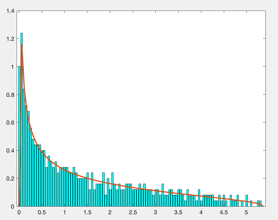
We are interested in the empirical spectral (eigenvalue) distribution of \(\hat{\mathbf{\Sigma}}_g\) and its limiting spectral distribution when \(p/n=c_n\to c\in(0,\infty)\). The result below is analogy to the Marchenko-Pastur-Law.
References
[1] Xin Dang, Hailin Sang, and Lauren Weatherall. Gini covariance matrix and its affine equivariant version. Statistical Papers, 60(3):641–666, 2019.
[2] Weiming Li, Qinwen Wang, Jianfeng Yao, and Wang Zhou. On eigenvalues of a high-dimensional spatial-sign covariance matrix. Bernoulli, 28(1):606–637, 2022. 2.